Drop Shape analysis using Python

This tutorial proposes a way of analyzing an image of a drop on a SLIPS surface. At the end of it, we will have gathered the important characteristics of the drop:

• its edge
• its base radius
• the position of the triple (oil-drop-vapor) point
• the apparent contact angles

Installing the needed packages

Basic packages

During this tutorial, we will need several python packages that has to be installed on your environment. The majority of the needed packages can be installed from PyPI using the following command:

pip install imageio matplotlib numpy scipy

Or for conda users:

conda install imageio matplotlib numpy scipy

OpenCV

We will also need OpenCV to be installed. For conda users on windows, you should be able to get this working with the following command:

conda install opencv

Or this one:

conda install -c menpo opencv

For Linux users, get OpenCV from your distribution repository or build it from source.

Importing images

Imageio package allows to import and export a variety of image formats (see here for an exhaustive list).

Imageio can also import videos or grab images directly from cameras.

import imageio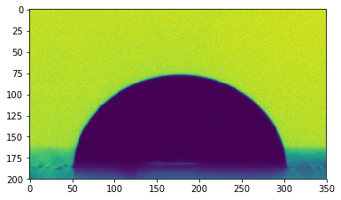
image = imageio.imread('data/image.bmp')

Images are stored as arrays of numbers. We can display them using the matplotlib package:

import matplotlib.pyplot as plt
plt.figure()
plt.imshow(image)
plt.colorbar()
plt.show()

<Figure size 640x480 with 2 Axes>

Cropping

The drop is centered on the image, but a part of the syringe that was used to drop it is also visible at the top.

An edge detection performed directly on this image will certainly detect the syringe edges. To avoid that, we will restrain the area of interest around the drop.

image = image[200:400, 200:550]

# Display
plt.figure()
plt.imshow(image)
plt.show()
              

Edge detection

OpenCV (Open Source Computer Vision Library) is a well-known library for image analysis that provides a Python interface. We will use one of its edge detection functions to get the edge of our drop. More specifically, we will use the Canny edge detector.

This edge detector method necessitates to specify two threshold values, that have to be optimized depending on the nature/quality of the edges to detect. A first good guess is generally to take the minimal and maximal pixel values as thresholds.

import cv2
thres1 = image.min()
thres2 = image.max()
edges = cv2.Canny(image, thres1, thres2)

# Display the edges
plt.figure()
plt.imshow(edges)
plt.show()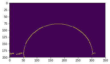

The Canny() function returns an array of numbers that is equal to 1 (in yellow here) where edges have been detected, and 0 (in blue here) elsewhere.

OpenCV successfully detects the drop edges, but also some structures near the sample surface. Lets improve the threshold values to get rid of those unwanted bits.

thres1 = image.min()*0.75
thres2 = image.max()*1.5
edges = cv2.Canny(image, thres1, thres2)

# Display the edges
plt.figure()
plt.imshow(edges)
plt.show()

We got rid of some of the unwanted bits, but we still detect some weird shapes due to the reflection of the drop on the sample (around x=50, y=200 for example). We can remove them by deleting all the edges detected below the baseline, that is here roughly y=180.

edges[180:, :] = 0

# Display the edges
plt.figure()
plt.imshow(edges)
plt.show()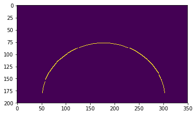

From image to points

Our drop edge is for the moment stored as an array of 0 and 1. If we want to access the edge coordinates, we need to find the positions of each pixel equal to 1 (yellow pixels here).

The numpy package can help us do that by detecting where the pixel values are not zero.

import numpy as np
ys, xs = np.where(edges)
ys = np.asarray(-ys, dtype=float)
xs = np.asarray(xs, dtype=float)

# Display the edges
plt.figure()
plt.plot(xs, ys, marker='o', ls='none')
plt.axis('equal')
plt.show()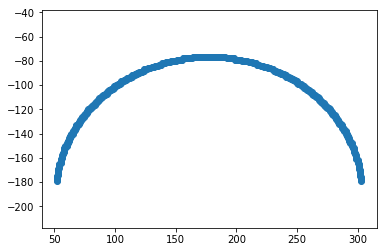

For convenience, we want to center the drop on the referential.

xs = xs - xs.mean()
ys = ys - ys.min()

# Plot the edges
plt.figure()
plt.plot(xs, ys, marker='o', ls='none')
plt.axhline(0, color='k')
plt.axis('equal')
plt.show()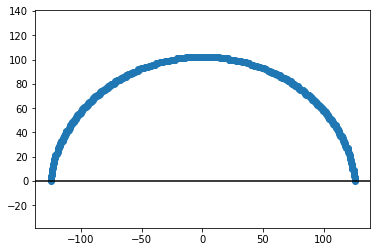

From pixels to mm

We achieved to get the edge coordinated in pixel. To pass this information into millimeters, we need to know the ratio between pixels and mm for our base image.

It can be done by measuring the syringe diameter (here ~60 pixels) that we know is about 0.5mm. This gives us a resolution of 120px/mm.

We can now scale our edge coordinates:

res = 120 
xs /= res
ys /= res

# Plot the edge
fig, axs = plt.subplots(1, 2, figsize=(10, 4))
plt.sca(axs[0])
plt.plot(xs, ys, marker='o', ls='none')
plt.axhline(0, color='k')
plt.axis('equal')
plt.xlabel('x [mm]')
plt.ylabel('y [mm]')
# Plot a zoom on the edge
plt.sca(axs[1])
plt.plot(xs, ys, marker='o', ls='none')
plt.axhline(0, color='k')
plt.axis('equal')
plt.xlabel('x [mm]')
plt.xlim(-1.15, -0.9)
plt.ylim(-0.05, 0.3)
plt.title("Zoom")
plt.show()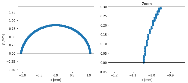

Fitting the edge

Problem with the edge coordinates we obtained at this point is that they are at discrete positions (because extracted from an image). It is impossible to obtain contact angles or triple point position from this kind of discretized data. In order to go further, we need to find a good fitting of the drop edge.

The Scipy package provides several ways of fitting different kind of data. Here, as we don’t care about the mathematical expression of our fitting, we will use a spline fitting: UnivariateSpline.

This fitting function needs the data to be sorted and with strictly increasing x values. Our edge coordinated need some transformation to fit those specifications.

# Ensure increasing x values
new_xs = np.sort(list(set(xs)))
new_ys = []
for x in new_xs:
    new_ys.append(np.mean(ys[xs == x]))
xs = new_xs
ys = np.asarray(new_ys)

# Fitting the drop edge
import scipy.interpolate as spint
edge_f = spint.UnivariateSpline(xs, ys, k=5, s=0.005)

# Display the fit
fig, axs = plt.subplots(1, 2, figsize=(10, 4))
plt.sca(axs[0])
plt.plot(xs, ys, marker='o', ls='none')
plt.plot(xs, edge_f(xs))
plt.axhline(0, color='k')
plt.xlabel('x [mm]')
plt.ylabel('y [mm]')
plt.axis('equal')
# Plot a zoom on the edge
plt.sca(axs[1])
plt.plot(xs, ys, marker='o', ls='none')
plt.plot(xs, edge_f(xs))
plt.axhline(0, color='k')
plt.axis('equal')
plt.xlabel('x [mm]')
plt.xlim(-1.1, -0.7)
plt.ylim(0, 0.5)
plt.title("Zoom")
plt.show()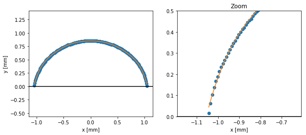

Getting the drop basic properties

We can now extract some information from our data, like the drop base length or the drop height:

base_radius = xs.max() - xs.min()
height = ys.max()

# Print
print("Drop base: {} mm".format(base_radius))
print("Drop height: {} mm".format(height))

Drop base: 2.091666666666667 mm
Drop height: 0.85 mm

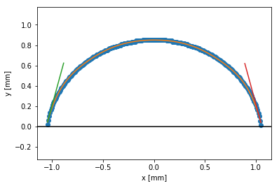
Getting the contact angles

The contact angles are the angles made by our fitted curve and the baseline (here y=0).

# Get left and right contact points
left_x = np.min(xs)
right_x = np.max(xs)
dx = (right_x - left_x)/100

# Left angle
import scipy.misc as spmisc
deriv = spmisc.derivative(edge_f, left_x, dx=dx)
theta_left =  np.arctan(deriv)

# Right angle
deriv = spmisc.derivative(edge_f, right_x, dx=dx)
theta_right = np.pi + np.arctan(deriv)

# Print
print(theta_left/np.pi*180)
print(theta_right/np.pi*180)

# Display the fit and the angles
plt.figure()
plt.plot(xs, ys, marker='o', ls='none')
plt.plot(xs, edge_f(xs))
plt.axhline(0, color='k')
angle_len = .6
plt.plot([left_x, left_x + angle_len*np.cos(theta_left)],
         [edge_f(left_x), edge_f(left_x) + angle_len*np.sin(theta_left)])
plt.plot([right_x, right_x + angle_len*np.cos(theta_right)],
         [edge_f(right_x), edge_f(right_x) + angle_len*np.sin(theta_right)])
plt.xlabel('x [mm]')
plt.ylabel('y [mm]')
plt.axis('equal')
plt.show()

74.74264462928066
105.21597243751776

Getting the triple point

Coming soon…